Inside mixture of experts, how sparse models decouple size from cost

A standard transformer is dense, which means that every one of its parameters participates in processing every token. The cost of a forward pass therefore scales directly with the size of the model, so the only way to make a dense model more capable, by making it larger, is also to make it proportionally more expensive to run. Every extra billion parameters is an extra billion multiplications on every single token, in training and again in serving. This is the wall that mixture of experts was invented to get around.

The idea is to make the computation conditional. Inside each layer, instead of one feed forward network that every token passes through, you place many of them side by side, each called an expert. A small network called the router looks at each token and decides which few experts should handle it. Only those experts do any work. The rest sit idle for that token. The model can therefore hold the combined knowledge of hundreds of experts while spending, on each token, only the compute of the handful it actually used. The size of the model and the cost of running it become two separate numbers, and almost everything interesting about the architecture follows from that separation.

A short history of a long idea

This is not a new invention, and it helps to see the lineage, because each step solved a problem the previous one exposed.

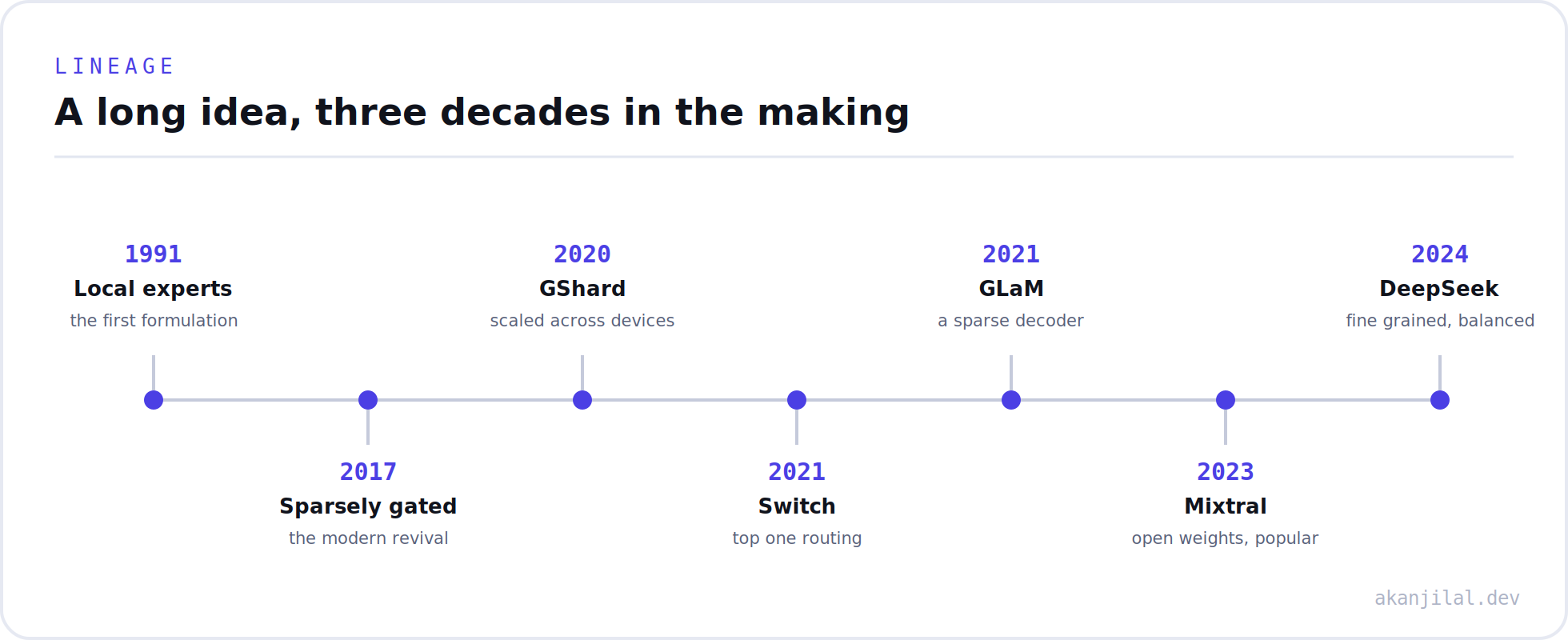
The idea dates to 1991, when Robert Jacobs, Michael Jordan, Steven Nowlan, and Geoffrey Hinton described what they called adaptive mixtures of local experts. The proposal was to train several small networks alongside a gating network that learns, for each input, which expert to trust. The experts would naturally divide the problem between themselves, each becoming good at a different part of it. The idea was elegant, and for decades it stayed mostly a curiosity, because the models of the time were small enough that conditional computation was not yet worth the trouble.

It returned at scale in 2017, when Noam Shazeer and colleagues published a paper with the memorable title about outrageously large neural networks. They placed a sparsely gated mixture of experts layer, with thousands of experts, between the recurrent layers of a language model, and showed that you could grow the capacity of a network enormously while keeping the compute per example almost flat. This was the modern revival, and it set the template that everything since has followed.

The next few years were about making it work at the scale of real systems. In 2020, the GShard work showed how to spread the experts of a single model across many accelerators and train a model with hundreds of billions of parameters for multilingual translation, which is when expert parallelism became a serious engineering discipline rather than a research idea. In 2021, the Switch Transformer simplified the routing all the way down to a single expert per token, which made the system cheaper and more stable and carried it to the trillion parameter scale. The same year, the GLaM model demonstrated the payoff for language modeling directly, holding more than a trillion parameters yet beating a much smaller dense model while using roughly half the compute. By late 2023, Mistral released Mixtral, which put a strong sparse model into everyone's hands as open weights and did a great deal to make the architecture mainstream. And through 2024 and into 2025, the DeepSeek family refined it further, with many small experts, always on shared experts, and a balancing method that needs no auxiliary penalty, which we will come to.

The anatomy of a mixture of experts layer

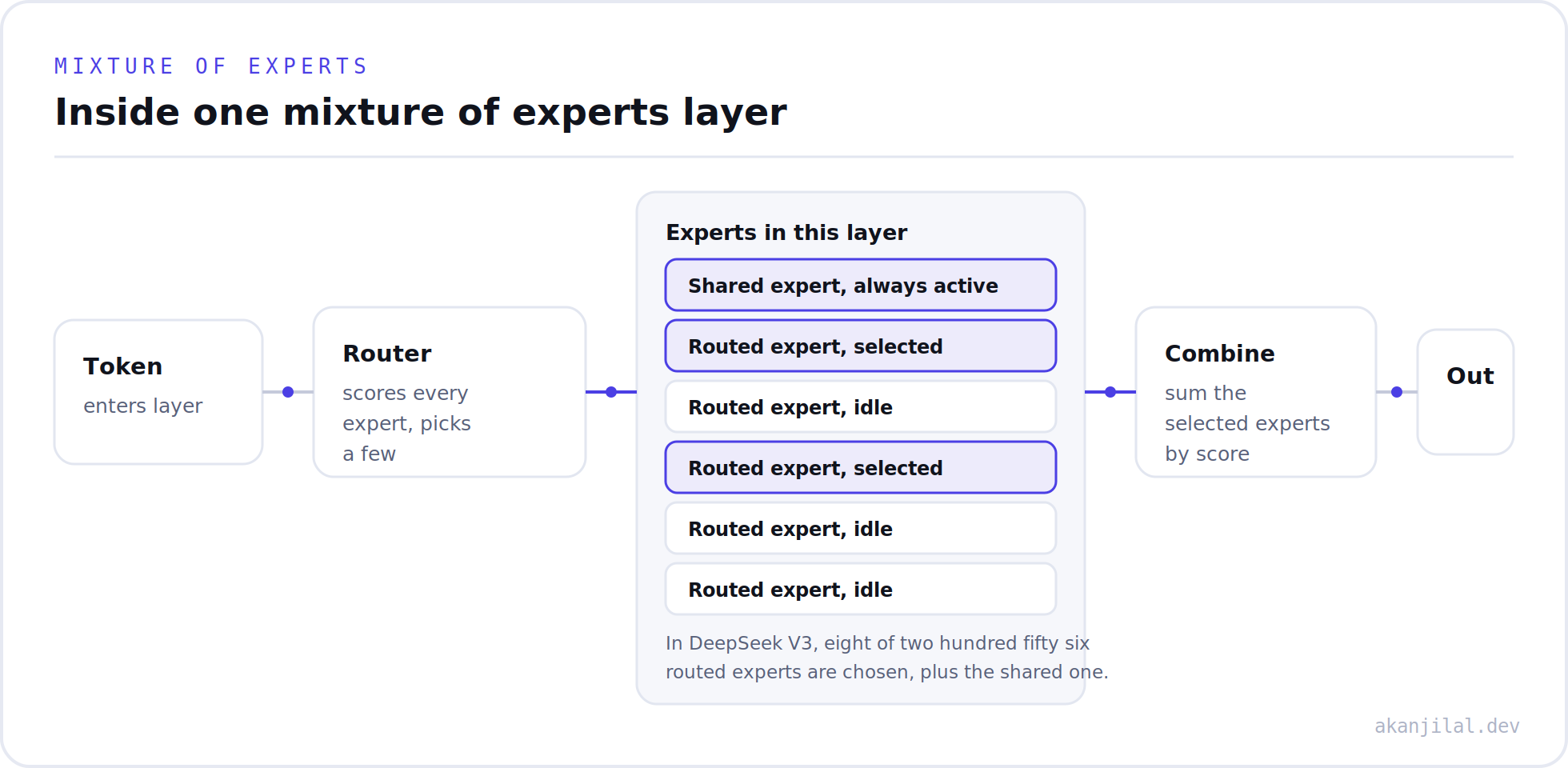
The mechanism lives inside the transformer block, in place of the ordinary feed forward network. Where a dense model has one such network that every token passes through, a sparse model has many of them, the experts, plus the small router that chooses between them. The router scores the experts for the current token, the few highest scoring experts each process the token, and their outputs are combined into one result weighted by the router's scores. Many modern designs also keep one or two shared experts that are always active for every token, which capture the common patterns that every token needs, leaving the routed experts free to specialize.

The gating computation, step by step

It is worth being precise about what the router actually does, because it is simpler than people expect and it is the heart of the whole architecture. The router is a small linear layer. For a given token, it produces one number for each expert, a score that says how well that expert suits this token. A softmax turns those raw scores into a set of probabilities that sum to one. The router then keeps only the few highest, a strategy known as top routing, where the number kept might be one, or two, or eight, depending on the design. The probabilities of the kept experts are rescaled so that they again sum to one among themselves, those experts each process the token, and their outputs are added together in proportion to those rescaled weights.

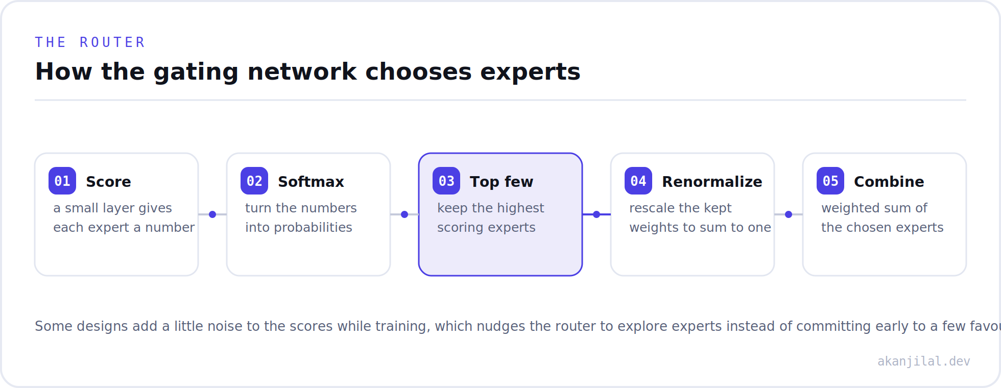
One refinement from the early work is worth knowing. Shazeer and colleagues found it helpful to add a little random noise to the scores during training. Without it, the router tends to commit too early to whichever experts happened to look good first, and it never gives the others a chance to improve. A touch of noise keeps the router exploring, which matters a great deal for the balancing problem we will reach shortly.

The economics, active against total

This is where the architecture earns its place, and where it connects to anything anyone cares about in production, which is cost. A mixture of experts model has two parameter counts that matter, and confusing them is the most common mistake people make when reasoning about these systems. The total parameter count is how many parameters the model has in all of its experts combined. The active parameter count is how many actually do work on a single token. The compute required for a forward pass, and therefore the cost and the latency of generation, scales with the active count, not the total.

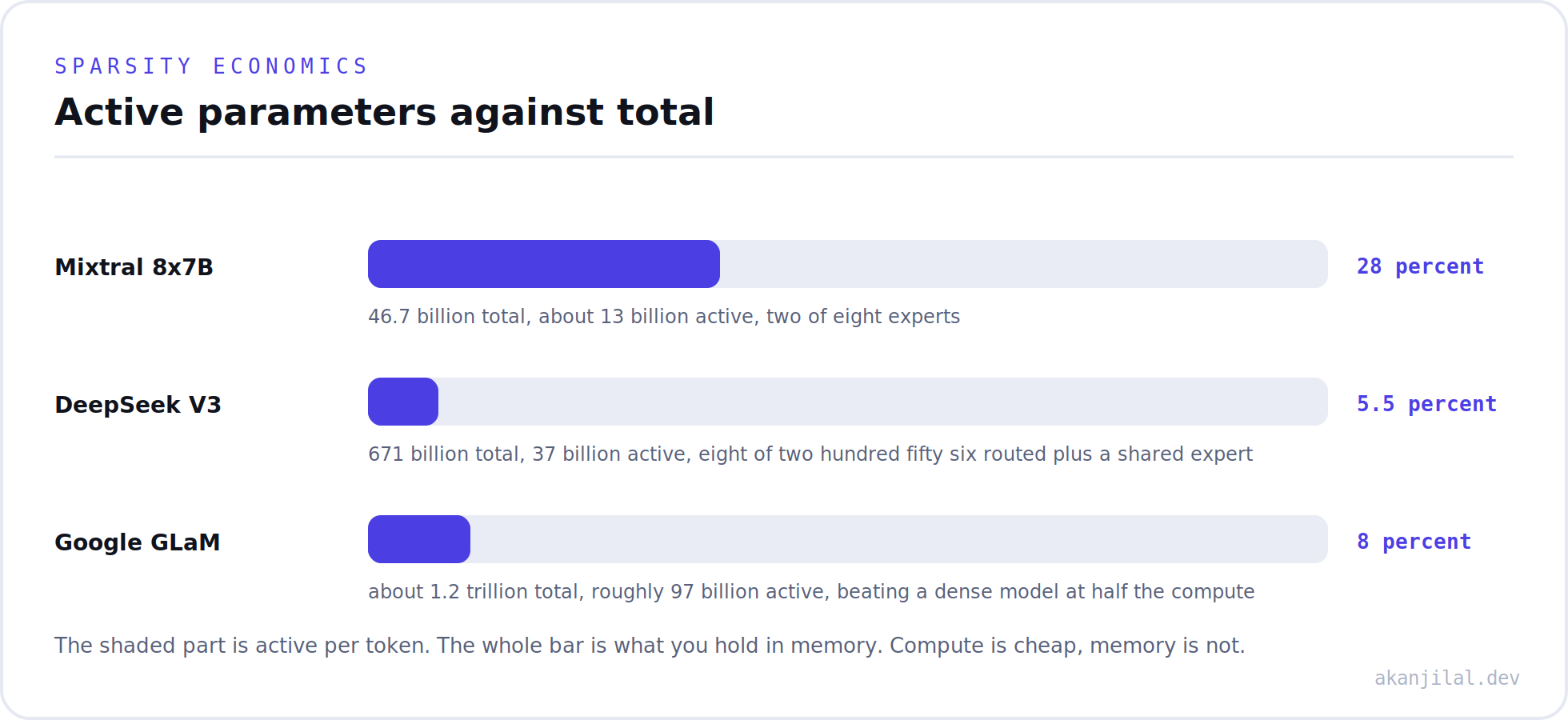
The numbers make the point concrete. Mistral's Mixtral, released in late 2023, holds about 46.7 billion parameters but activates only around 13 billion for each token, by selecting two of its eight experts, and at that cost it matched the quality of a dense model with seventy billion parameters while running several times faster. DeepSeek V3, released a year later, holds 671 billion parameters and activates only 37 billion, roughly one eighteenth of the model, by choosing eight of two hundred and fifty six routed experts and adding one shared expert. Google's earlier research model, known as GLaM, held more than a trillion parameters and beat a dense model many times smaller while using about half the compute. In every case the model has the capacity of a much larger network while incurring the compute cost of a smaller one.

Fine grained experts, and a shared one

A subtle design choice has a large effect on quality. Rather than a few large experts, recent architectures use many small ones, a technique called fine grained expert segmentation. The idea, introduced in the DeepSeek work on the subject, is to split each expert into several smaller ones and activate proportionally more of them, which keeps the total compute identical while giving the router far more combinations to choose from. If you turn one expert into four smaller ones and activate four where you used to activate one, the arithmetic is unchanged, but the number of distinct ways to combine experts grows enormously. More combinations means each expert can specialize more narrowly, and research has shown that this finer granularity buys meaningfully better quality at the same active parameter count.

The shared expert is the complement to this idea. Some knowledge is needed for almost every token, such as the basic shape of grammar, and it would be wasteful for many routed experts to each learn it separately. So one or two experts are marked as always active, processing every token regardless of routing, which lets them absorb the common knowledge and frees the routed experts to capture what is distinctive. It is worth being precise about what specialization means here, because the intuition is usually wrong. Experts do not divide up neatly by subject, so there is no coding expert and no French expert. The specialization happens at the level of individual tokens within individual layers, and it is a statistical tendency rather than a clean, human readable partition.

Two ways to route, token choice and expert choice

So far the router has worked the obvious way. Each token looks at the experts and chooses the few it wants. This is called token choice routing, and it is the default in most models, including Mixtral and the DeepSeek family. It is simple and it works, but it has a structural weakness. Nothing stops a popular expert from being chosen by far more tokens than its neighbours, which leaves some experts overloaded and others barely used, and that imbalance is both wasteful and unstable.

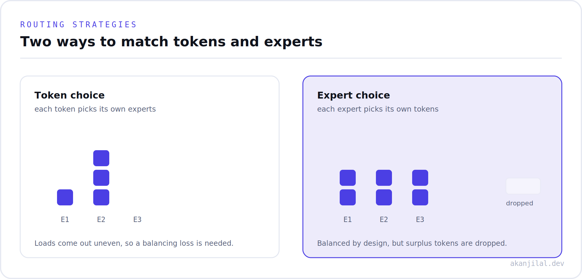
In 2022, a team at Google proposed inverting the decision, in work presented at the Neural Information Processing Systems conference under the name expert choice routing. Instead of each token picking its experts, each expert picks its tokens. Every expert is given a fixed budget, called its capacity, and it selects the tokens that score highest for it, up to that budget. The beautiful consequence is that the load is now perfectly balanced by construction, because every expert processes exactly the same number of tokens, and no auxiliary balancing penalty is needed at all.

That budget is set by a value called the capacity factor, which is roughly the average number of experts each token gets to use. It introduces a new wrinkle. If a token is not among the highest scoring choices for any expert that still has room, it is simply not processed by any expert in that layer, which is called token dropping. This sounds alarming, and in practice it is softened by the fact that transformer layers have residual connections, so a dropped token still carries its previous representation forward rather than vanishing. The honest summary is that the two strategies trade one problem for another. Token choice can imbalance the load, and expert choice can skip tokens, and a great deal of the recent research on routing is about getting the benefits of both at once.

The hard part, keeping the experts balanced

For the common token choice models, the imbalance problem has to be managed directly, and it is one of the central engineering challenges of training these systems. If you simply let the router learn freely, it tends to collapse onto a few favorite experts, sending most tokens to them while the rest barely train. The idle experts are dead capacity you paid for, and the favored ones become a bottleneck.

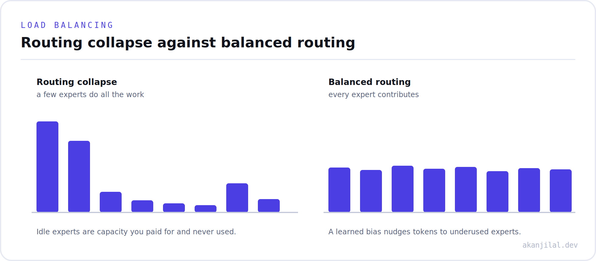
The traditional fix was to add an auxiliary loss during training, an extra penalty that punishes the model whenever the experts are used unevenly. It works, but it creates a tension, because the model is now being optimized for two goals at once, getting the answer right and spreading the load evenly, and those goals sometimes pull against each other and destabilize training. A related stabilizer, introduced in the work on stable and transferable sparse models, is a small penalty on the size of the router's raw scores, sometimes called the router z loss, which stops those scores from growing large enough to make the softmax numerically fragile. Together these kept large sparse models trainable, but they were always a little awkward.

DeepSeek V3 introduced a cleaner approach that drops the auxiliary loss almost entirely. Instead, it gives each expert a small bias term that is added to the router's scores, and that bias is nudged up when the expert is underused and down when it is overloaded. The routing decision itself stays focused purely on quality, while the bias quietly keeps the load even in the background, and the reported result was dramatically more stable training with no irrecoverable loss spikes across an enormous run. It is a small idea with a large payoff, and a good example of how much of the recent progress in these systems comes from careful engineering of the training dynamics rather than from raw scale.

Serving them, where communication is the hidden cost

In production, the experts of a large model do not fit on a single accelerator, so they are spread across many, a setup called expert parallelism. This turns routing into a networking problem as much as a computation one. Twice in every layer, the system performs an all to all exchange. First it dispatches each token to whichever device holds the expert it was routed to, and then, once the experts have done their work, it gathers the results back. At large scale, these exchanges, not the arithmetic inside the experts, become the dominant cost, and a great deal of systems engineering goes into balancing the communication so that no single link or device becomes the bottleneck.

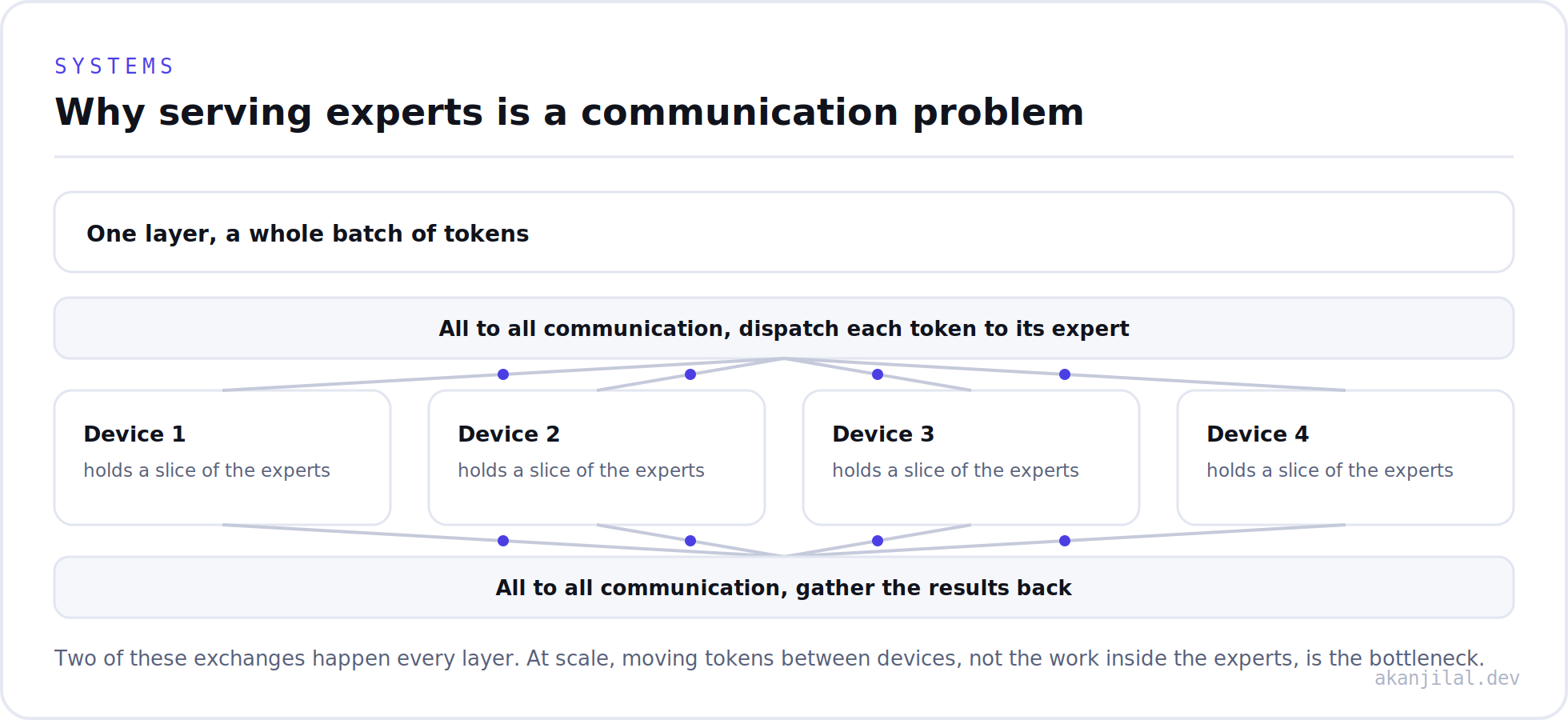
This systems view also explains two facts that surprise people. The first is why these models are usually run at high batch sizes. Spreading many tokens across the experts at once is what keeps every device busy, so the economics improve as the batch grows, which is the opposite of the intuition that a bigger model should be slower per request. The second is why memory dominates the cost of ownership. Because every expert must be held resident in case the router calls on it, a sparse model occupies the memory of a very large model even though it computes like a small one, which is why so much effort goes into quantizing the experts to make them smaller in memory without changing the routing.

When mixture of experts is worth it, and when it is not

It would be a mistake to read all of this as an argument that sparse beats dense in every case. The architecture is a scaling tool, and like any tool it fits some situations and not others. It is at its best when you are serving a very capable model at scale, where you can amortize the large memory footprint across a steady stream of batched requests and the savings in compute are substantial and continuous. It is also the practical way to train a frontier quality model on a constrained compute budget, which is exactly what the DeepSeek results demonstrated.

It is a poorer fit in a few situations that are worth naming honestly. A small deployment that cannot keep all of the experts resident cheaply loses the very advantage that justifies the architecture, since you pay the full memory cost without the scale to amortize it. Fine tuning a sparse model is trickier than fine tuning a dense one, because the routing and its balance have to be preserved, and a naive fine tune can unbalance the experts or overfit the few that a small dataset happens to activate. And a latency sensitive path that handles one request at a time, with little opportunity to batch, will not see the throughput benefit that makes the memory cost worthwhile. None of these are reasons to avoid the architecture. They are reasons to choose it deliberately, for the workloads where its particular economics actually pay off.

The architect's view

Step back, and the lesson is one an architect will recognize from any other domain. Mixture of experts is conditional computation, the same principle as only loading the code path you need, only querying the index you must, only spending the resource the request actually requires. It decouples the thing you are tempted to measure, the total size, from the thing that actually costs you, the active work, and it pays for that decoupling with memory and with the engineering of routing and balance. The teams who reason clearly about these models are the ones who keep those two numbers separate, who remember that memory and compute scale differently, who choose the routing strategy with eyes open to its failure mode, and who treat the router and its balance as a first class part of the system rather than an implementation detail. Get those things right, and you can serve a model with very high capacity at a compute cost well below what its total parameter count would suggest.

References

- Robert Jacobs, Michael Jordan, Steven Nowlan, and Geoffrey Hinton, Adaptive Mixtures of Local Experts, Neural Computation (1991).https://doi.org/10.1162/neco.1991.3.1.79
- Noam Shazeer and colleagues, Outrageously Large Neural Networks, the Sparsely Gated Mixture of Experts Layer (2017).https://arxiv.org/abs/1701.06538
- Dmitry Lepikhin and colleagues, GShard, Scaling Giant Models with Conditional Computation and Automatic Sharding (2020).https://arxiv.org/abs/2006.16668
- William Fedus, Barret Zoph, and Noam Shazeer, Switch Transformers (2021).https://arxiv.org/abs/2101.03961
- Nan Du and colleagues, GLaM, Efficient Scaling of Language Models with Mixture of Experts (2021).https://arxiv.org/abs/2112.06905
- Yanqi Zhou and colleagues, Mixture of Experts with Expert Choice Routing (2022).https://arxiv.org/abs/2202.09368
- Barret Zoph and colleagues, ST-MoE, Designing Stable and Transferable Sparse Expert Models (2022).https://arxiv.org/abs/2202.08906
- Mistral, Mixtral of Experts (2024).https://arxiv.org/abs/2401.04088
- Damai Dai and colleagues, DeepSeekMoE, towards ultimate expert specialization in mixture of experts language models (2024).https://arxiv.org/abs/2401.06066
- DeepSeek AI, DeepSeek V3 Technical Report (2024).https://arxiv.org/abs/2412.19437